AC Survey
Data summary
Main Variables
##  [1] "ivr_mobile_number"        "age"
##  [3] "gender"                   "audience_name"
##  [5] "ivr_response_status"      "ivr_response_status_name"
##  [7] "ac_name"                  "pc_name"
##  [9] "district_name"            "state_name"
## [11] "q1_response"              "q2_response"
Variable summary
| state_name | n_call | n_ac | n_pc | q1_response_rate | q2_response_rate | q1_and_q2_response_rate | q1_or_q2_response_rate |
|---|---|---|---|---|---|---|---|
| Gujarat | 21112 | 170 | 26 | 2.73 | 2.90 | 1.87 | 3.76 |
| Rajasthan | 31314 | 198 | 25 | 7.49 | 9.22 | 5.97 | 10.74 |
| Telangana | 28027 | 91 | 15 | 9.43 | 9.65 | 7.25 | 11.83 |
| Uttar Pradesh | 15090 | 393 | 80 | 5.88 | 7.67 | 4.63 | 8.91 |
| West Bengal | 19195 | 284 | 42 | 4.68 | 5.70 | 3.44 | 6.94 |
| state_name | mean_call_ac | mean_q1_or_q2_response_ac | mean_age_ac | mean_male_pc |
|---|---|---|---|---|
| Gujarat | 124.19 | 4.67 | NaN | NA |
| Rajasthan | 158.15 | 16.99 | 45.73 | 74.87 |
| Telangana | 307.99 | 36.44 | 36.74 | 66.56 |
| Uttar Pradesh | 38.40 | 3.42 | 37.85 | 84.06 |
| West Bengal | 67.59 | 4.69 | 25.04 | 44.71 |
States
Calls & Responses
States
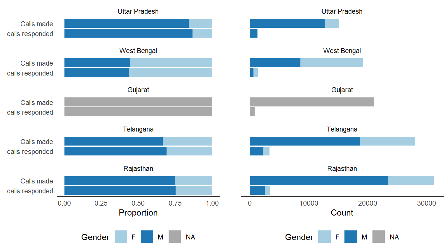
The following plot shows the proportion and the number of calls made and responded in each state along with the break-up of the gender. It is evident that, there is a huge gender bias in the calls made in the all three states except West Bengal. Also, among the four states, Uttar Pradesh seems to have received the least number of calls contradicting its population size.
Throughout the analysis, we count a responded call as the ones that have answered at least one of the two questions. It is quite evident that the number of respondents is relatively much less, averaging around 5% of the calls made. At the same time, the gender proportion of the respondents is identical to the callers.
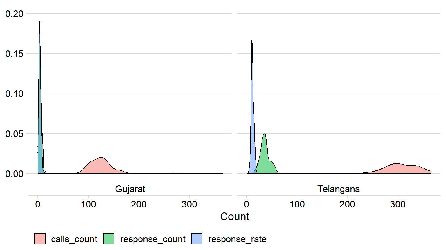
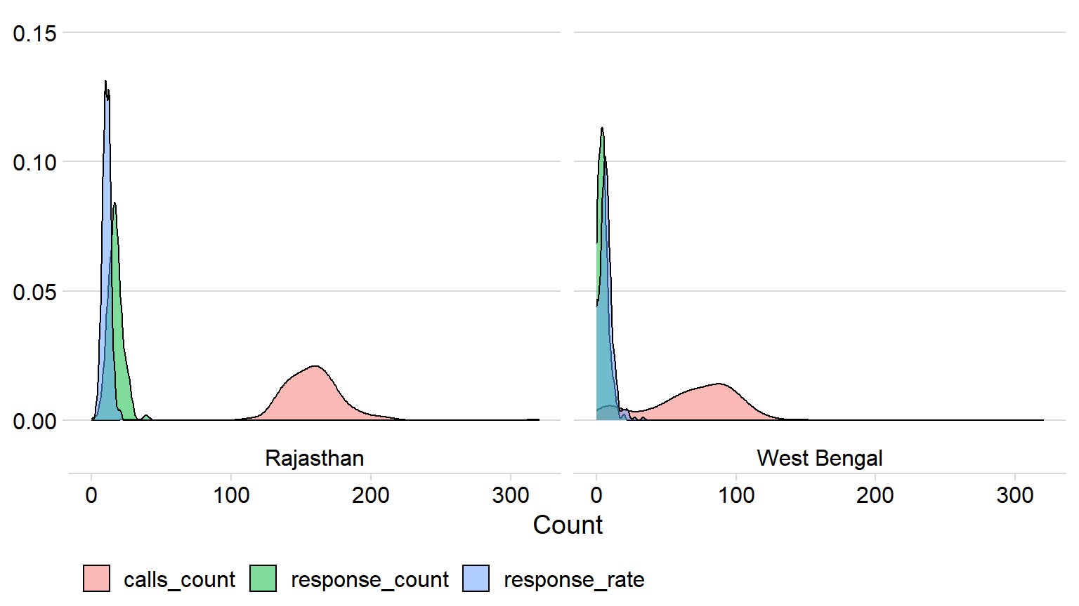
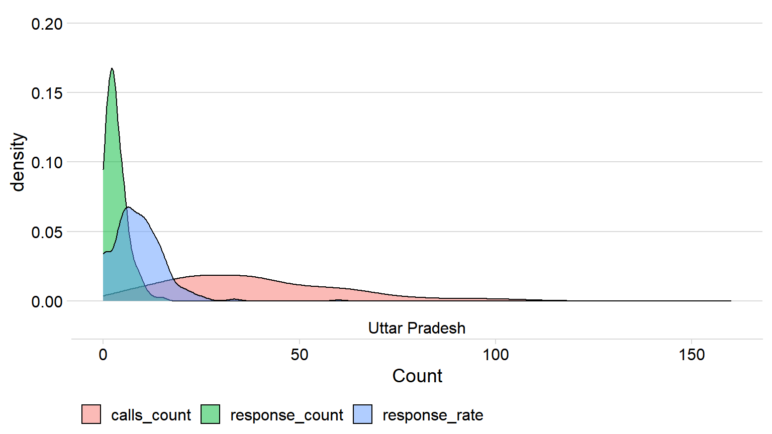
We use density plots to observe the distribution and the differences of Number of calls , Number of responses and the Response rate. among the states. Response rate is simply the percentage of the calls that received response to at least one of the the two questions. We observe significant variation among the states on all three variables.
Assembly constituencies
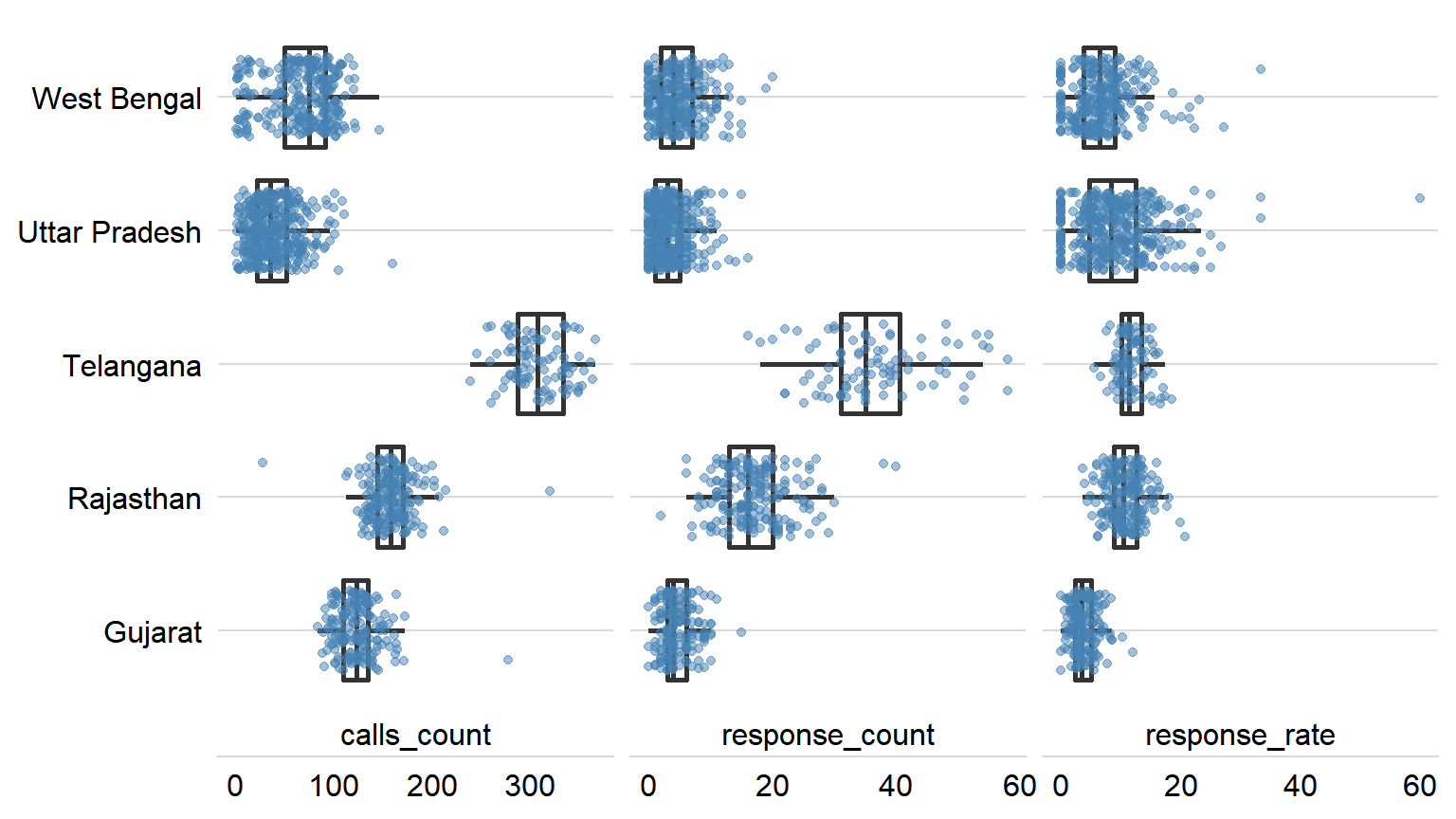
We explore the variation within the state by looking at the assembly constituency level.The following box plots illustrates the distribution of the calls, response and the response rate in all unique assembly constituencies in each state. The jittered dots represents the relavant value of the variables in every unique constituency in each states.
Gender
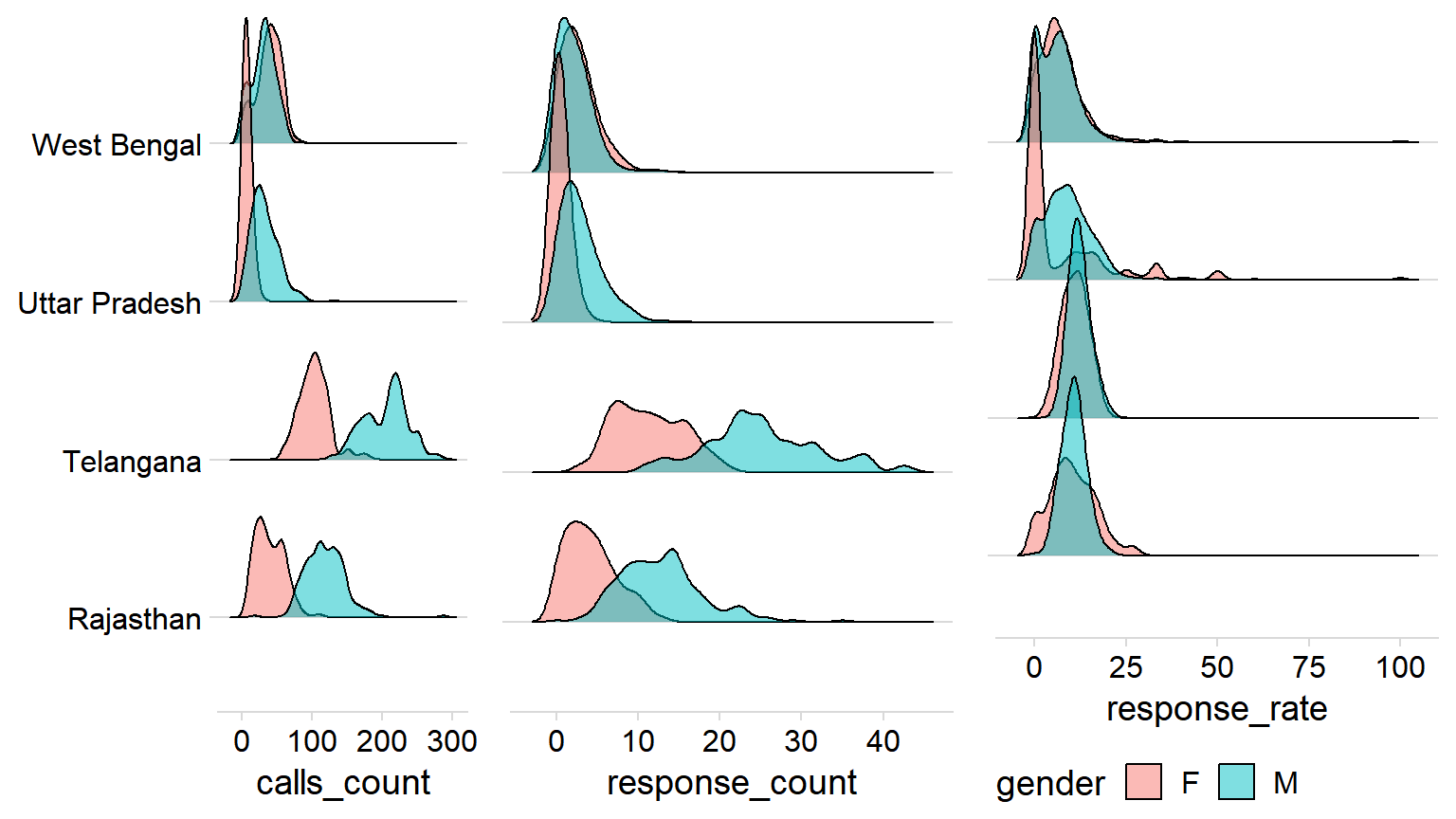
Density plots along the lines of gender does reflect the sample bias in the gender as expected . Telengana and Rajasthan have a fair distribution given we take the sample bias into account while Uttar Pradesh has a inconsistent distribution. West Bengal seems to have a symmetrical distribution.
–
Age
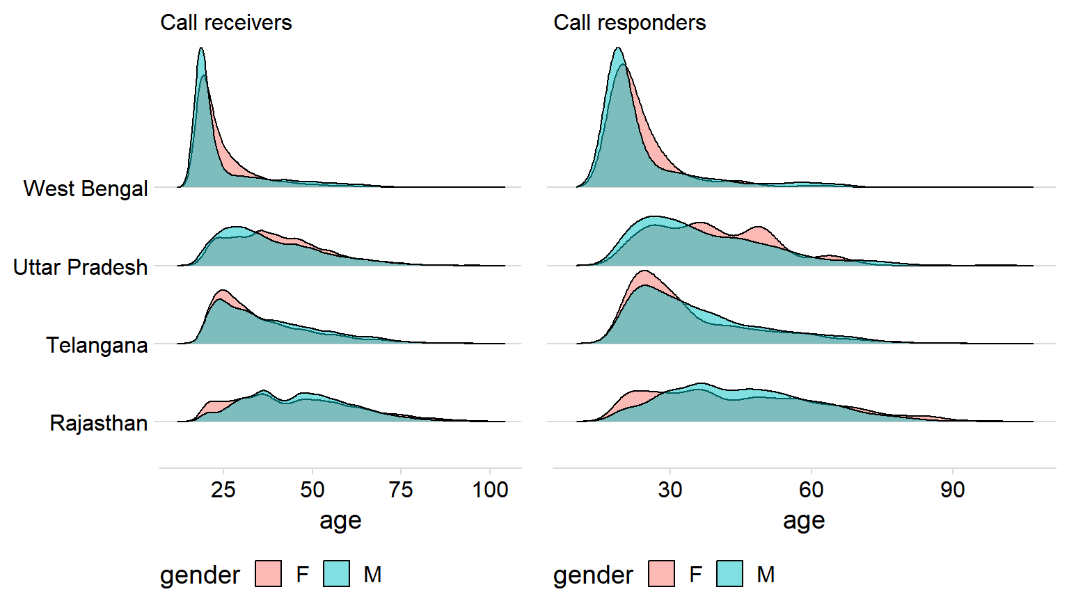
The following plot depicts the age distribution along with gender of the the callers. Looking at the aggregate picture, we observe that the proportion of calls to individuals less than 25 years is quite high among women.
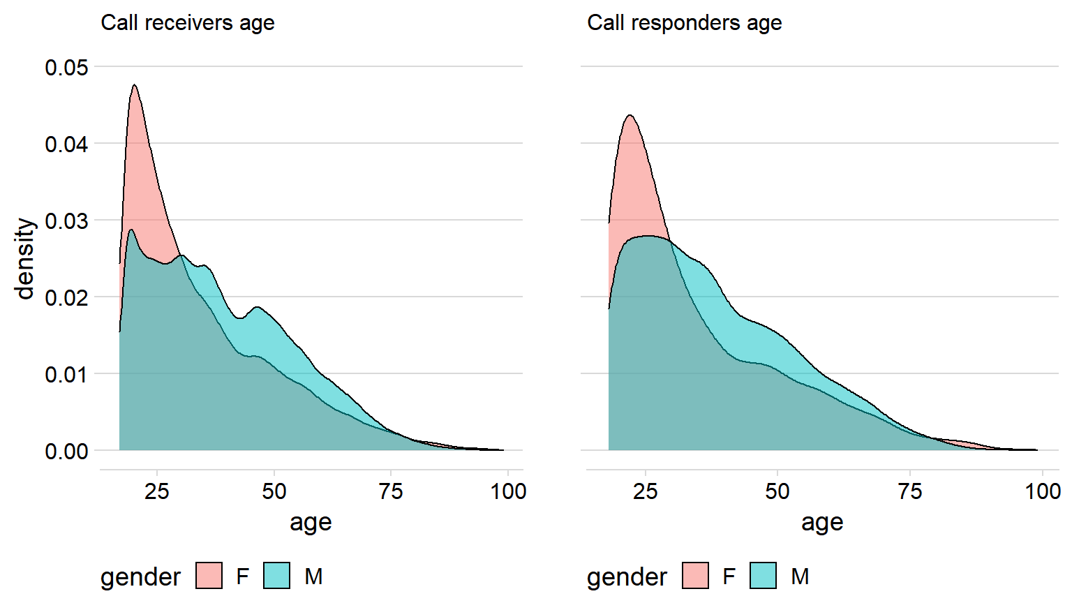
Once we look further into the states, the general trend fades away and looks more like the gender is fairly distributed along the age across the states. All the states except West Bengal has a fair distribution of age among both genders, while West Bengal one is extremely right skewed with a high number of young responders under 25 years of age.
Demography
Urban
In this section, we are attempting to ensure that there is no urban/rural bias in the sample. We define urban ACs as the constituencies with more than 40% of urban areas. The distribution of urban/rural ACs in the dataset looks like this.
| state_name | urban_y | count | n_ac | calls_per_ac | response_per_ac | response_rate_per_ac |
|---|---|---|---|---|---|---|
| Gujarat | 0 | 11318 | 85 | 133.15 | 5.25 | 3.94 |
| Gujarat | 1 | 5438 | 47 | 115.70 | 4.51 | 3.90 |
| Rajasthan | 0 | 27612 | 170 | 162.42 | 17.58 | 10.82 |
| Rajasthan | 1 | 3688 | 26 | 141.85 | 14.54 | 10.25 |
| Uttar Pradesh | 0 | 13522 | 335 | 40.36 | 3.54 | 8.76 |
| Uttar Pradesh | 1 | 1381 | 53 | 26.06 | 2.53 | 9.70 |
| West Bengal | 0 | 14525 | 210 | 69.17 | 5.07 | 7.33 |
| West Bengal | 1 | 4085 | 63 | 64.84 | 3.78 | 5.83 |
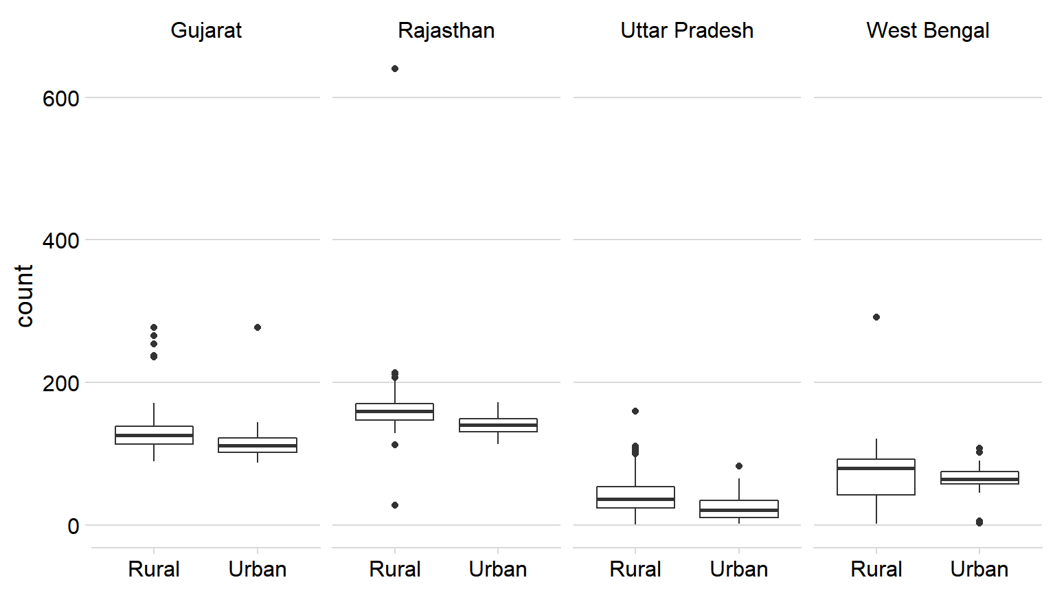
Calls
We see that both mean values and calls per constituency is considerably less for urban constituencies. We scrutinise this further by looking at a box plot.
Response rate
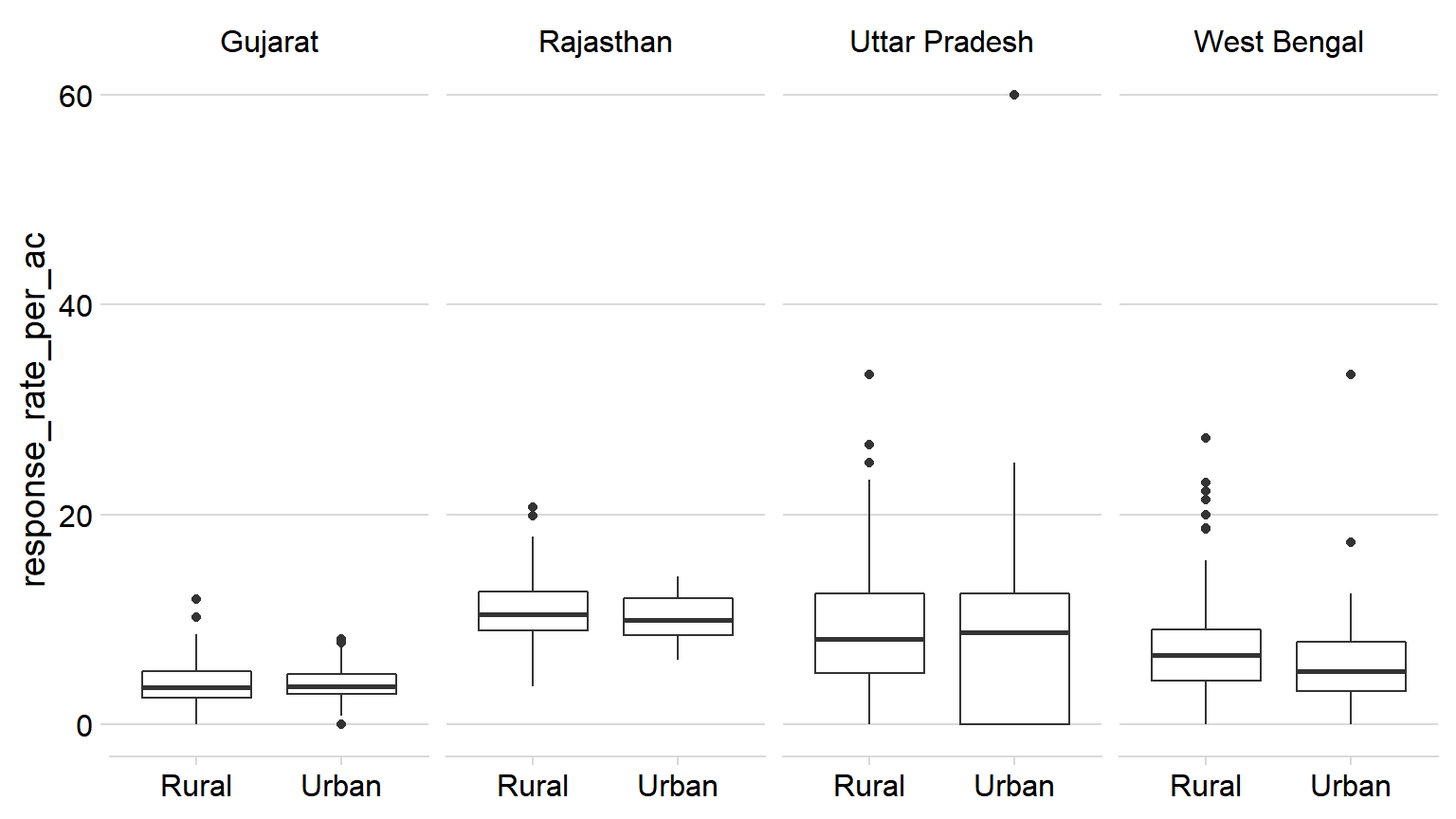
It seems that there is a rural bias in the sampling even though the response rate from urban and rural area looks similar. We can statistically confirm this using a t-test.
##
## 	Welch Two Sample t-test
##
## data:  survey_all_urban$count by survey_all_urban$urban_y
## t = 24.685, df = 22658, p-value < 2.2e-16
## alternative hypothesis: true difference in means is not equal to 0
## 95 percent confidence interval:
##  15.10509 17.71079
## sample estimates:
## mean in group 0 mean in group 1
##        126.7733        110.3653
We observe that there is a difference in the mean’s of both urban and rural constituencies and it is significant at .005 level. Hence, it is safe to conclude that there is a rural bias in the sample.
SC/ST
In the following table, sample_prop is the proportion of calls made to the that particular category and the electorate_prop is the electorate proportion of that category.
| State_Name | reservation | electorate_prop | state_name | calls_prop | response_prop |
|---|---|---|---|---|---|
| Gujarat | GEN | 0.79 | Gujarat | 0.93 | 0.94 |
| Gujarat | SC/ST | 0.21 | Gujarat | 0.07 | 0.06 |
| Rajasthan | GEN | 0.71 | Rajasthan | 0.70 | 0.69 |
| Rajasthan | SC/ST | 0.29 | Rajasthan | 0.30 | 0.31 |
| Uttar_Pradesh | GEN | 0.79 | Uttar Pradesh | 0.77 | 0.77 |
| Uttar_Pradesh | SC/ST | 0.21 | Uttar Pradesh | 0.23 | 0.23 |
In both UP and Rajasthan, there is a fair representation of SC/ST community in the calls made and responses received. But, in Gujarat, representation of SC/ST in this samples falls way below of their electoral proportion.
Answers
This analysis only includes only individuals who have atleast responded either one of the two questions.
All India
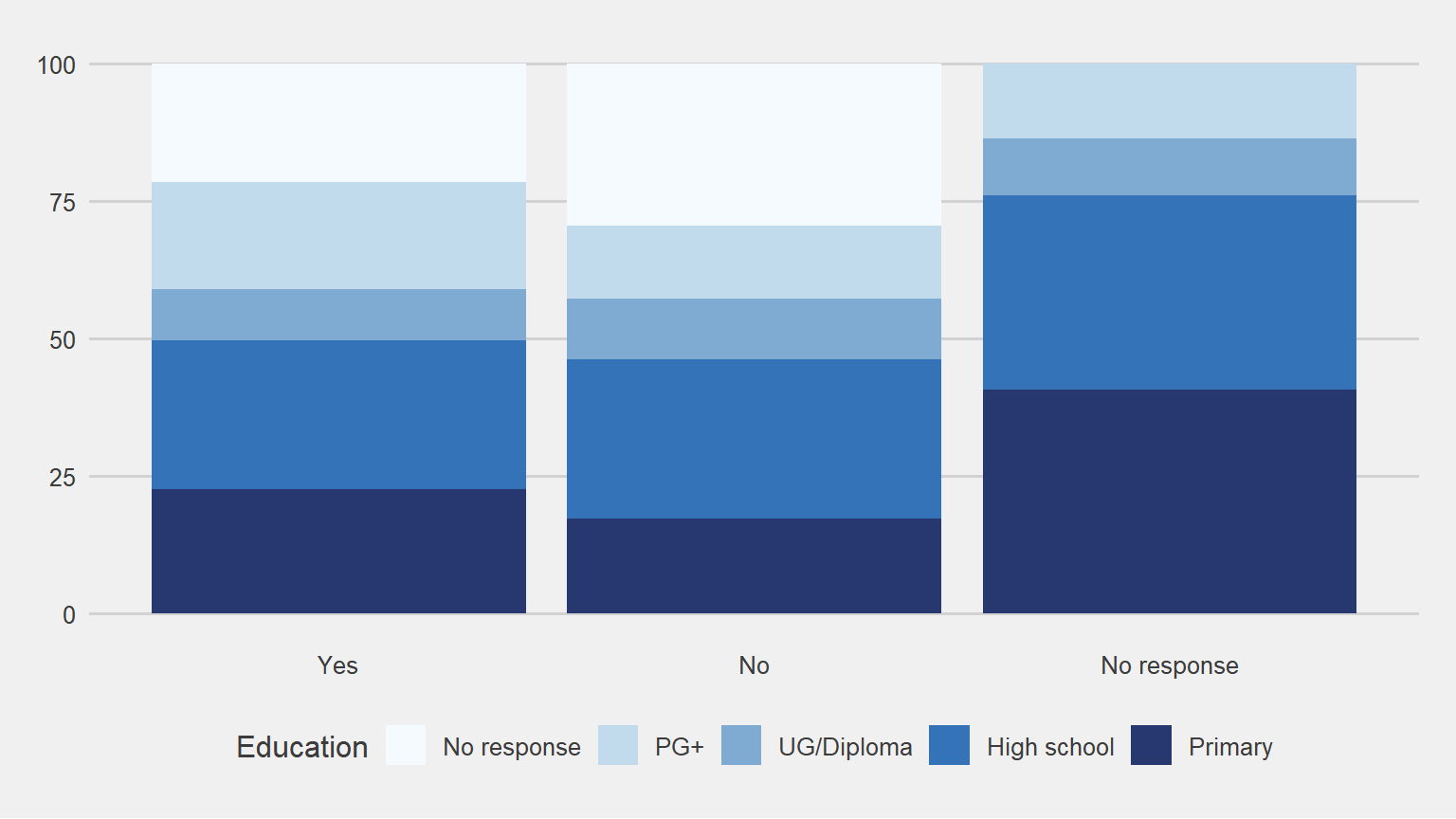
Education
In this grapph, we look at how people’s response differes with their education levels.
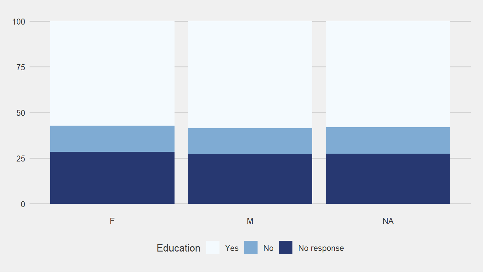
Gender
Here, we check if we observe any difference in the answers with regards to gender. As we can see, clearly there no difference along the gender lines.
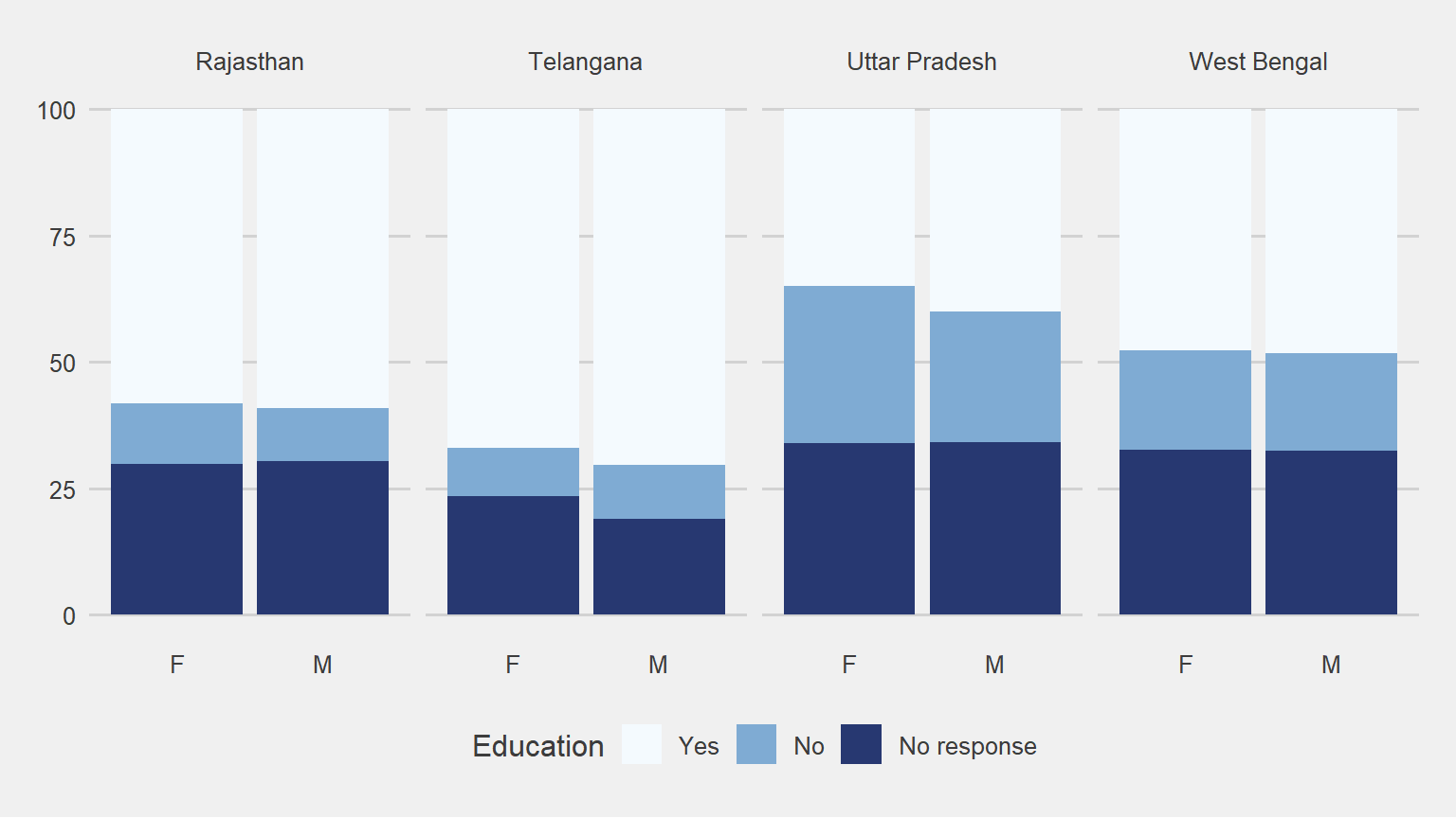
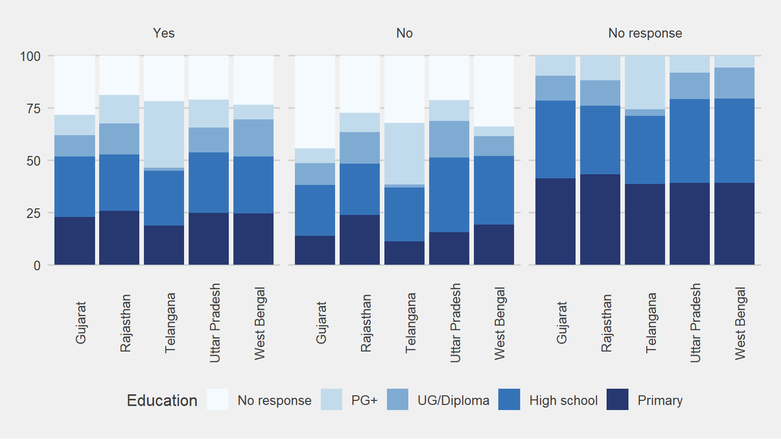
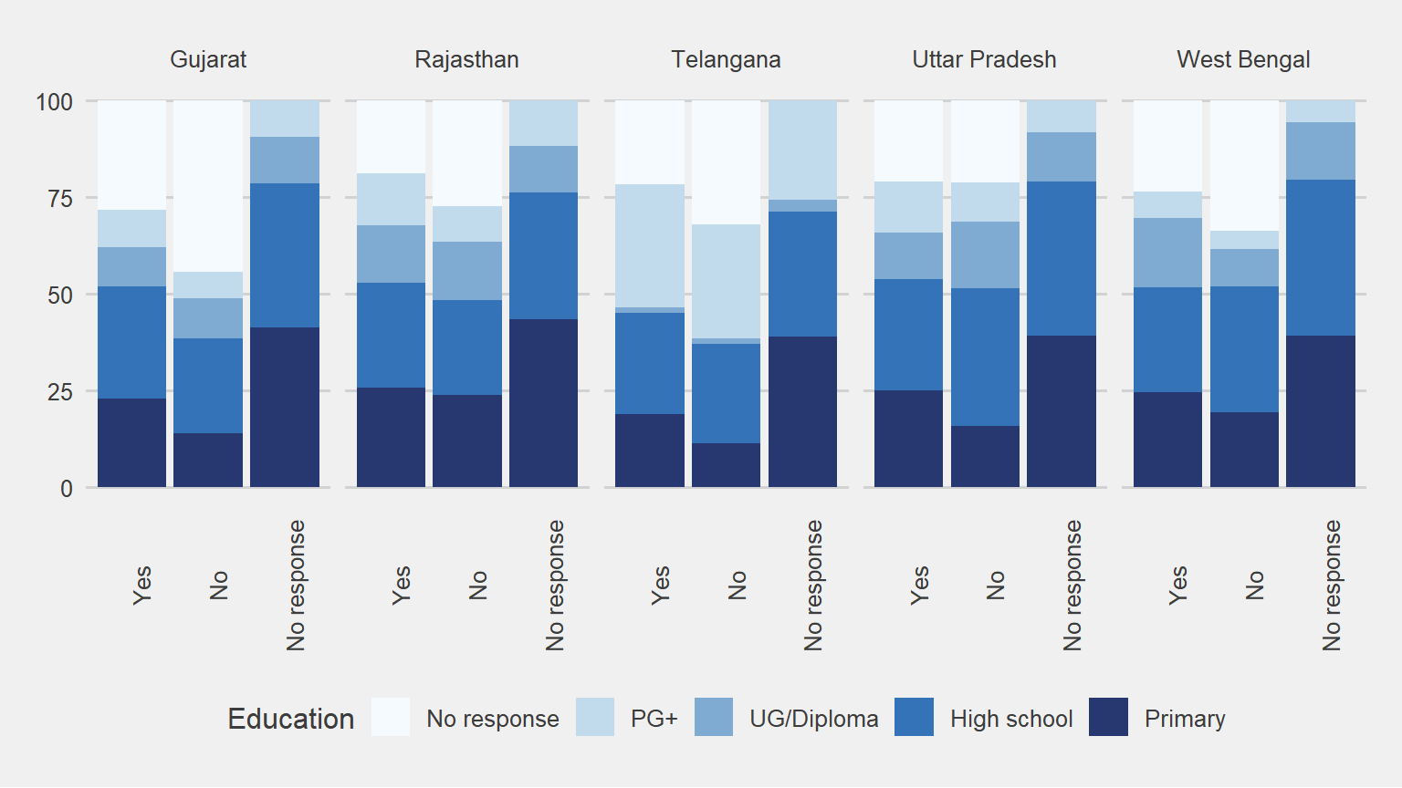
States
In the following charts, we observe how answers variate in different states with regards to education and gender.
Gender